Importing data

url <- 'http://www.equality-of-opportunity.org/data/college/mrc_table1.csv'
ratings <- readr::read_csv(url)

## Parsed with column specification:
## cols(
##   super_opeid = col_integer(),
##   name = col_character(),
##   czname = col_character(),
##   state = col_character(),
##   par_median = col_integer(),
##   k_median = col_integer(),
##   par_q1 = col_double(),
##   par_top1pc = col_double(),
##   kq5_cond_parq1 = col_double(),
##   ktop1pc_cond_parq1 = col_double(),
##   mr_kq5_pq1 = col_double(),
##   mr_ktop1_pq1 = col_double(),
##   trend_parq1 = col_double(),
##   trend_bottom40 = col_double(),
##   count = col_double()
## )

But the column names are not useful:

ratings %>% colnames

##  [1] "super_opeid"        "name"               "czname"            
##  [4] "state"              "par_median"         "k_median"          
##  [7] "par_q1"             "par_top1pc"         "kq5_cond_parq1"    
## [10] "ktop1pc_cond_parq1" "mr_kq5_pq1"         "mr_ktop1_pq1"      
## [13] "trend_parq1"        "trend_bottom40"     "count"

Exploring CUNY

Unfortunately, there is no yes/no column that tells us if a school is in CUNY or not.

Let’s start by a simple filter then. We will use the

ratings %>%
  filter(stringr::str_detect(name, 'Baruch'))

## # A tibble: 1 x 15
##   super_opeid name      czname state par_median k_median par_q1 par_top1pc
##         <int> <chr>     <chr>  <chr>      <int>    <int>  <dbl>      <dbl>
## 1        7273 CUNY Ber… New Y… NY         42800    57600   27.6      0.559
## # ... with 7 more variables: kq5_cond_parq1 <dbl>,
## #   ktop1pc_cond_parq1 <dbl>, mr_kq5_pq1 <dbl>, mr_ktop1_pq1 <dbl>,
## #   trend_parq1 <dbl>, trend_bottom40 <dbl>, count <dbl>

So maybe the way to get the CUNY schools is to filter for “CUNY”! Let’s give that a try:

ratings %>%
  filter(stringr::str_detect(stringr::str_to_upper(name), 'CUNY'))

## # A tibble: 16 x 15
##    super_opeid name     czname state par_median k_median par_q1 par_top1pc
##          <int> <chr>    <chr>  <chr>      <int>    <int>  <dbl>      <dbl>
##  1        7273 CUNY Be… New Y… NY         42800    57600   27.6     0.559 
##  2        2688 City Co… New Y… NY         35500    48500   32.5     0.234 
##  3        7022 CUNY Le… New Y… NY         32500    40700   36.7     0     
##  4        2693 CUNY Jo… New Y… NY         41800    45200   27.2     0.0979
##  5        2687 CUNY Br… New Y… NY         52200    44300   23.2     0.786 
##  6        2689 CUNY Hu… New Y… NY         49800    44400   21.2     0.561 
##  7        2690 CUNY Qu… New Y… NY         63300    48200   20.1     1.27  
##  8        4759 CUNY Yo… New Y… NY         36500    36400   30.7     0.0612
##  9        8611 CUNY, H… New Y… NY         26700    27700   45.8     0.0506
## 10        2691 CUNY Bo… New Y… NY         33500    31900   35.1     0.103 
## 11       10051 CUNY La… New Y… NY         33800    31800   36.8     0.0332
## 12        2692 CUNY Br… New Y… NY         29700    28700   41.0     0.0917
## 13        2697 Queensb… New Y… NY         42200    32400   27.6     0.0634
## 14       10097 CUNY Me… New Y… NY         35100    30900   30.5     0.137 
## 15        2694 Kingsbo… New Y… NY         40700    31300   27.1     0.161 
## 16        2698 College… New Y… NY         73500    41200   14.3     0.355 
## # ... with 7 more variables: kq5_cond_parq1 <dbl>,
## #   ktop1pc_cond_parq1 <dbl>, mr_kq5_pq1 <dbl>, mr_ktop1_pq1 <dbl>,
## #   trend_parq1 <dbl>, trend_bottom40 <dbl>, count <dbl>

There are more than 16 schools in CUNY but this will work for now.

Let’s order CUNY schools by their mobility ratings, highest to lowest:

ratings %>%
  filter(stringr::str_detect(stringr::str_to_upper(name), 'CUNY')) %>% 
  select(name, mr_kq5_pq1) %>%
  arrange(-mr_kq5_pq1) %>%
  head(10)

## # A tibble: 10 x 2
##    name                                        mr_kq5_pq1
##    <chr>                                            <dbl>
##  1 CUNY Bernard M. Baruch College                   12.9 
##  2 City College Of New York - CUNY                  11.7 
##  3 CUNY Lehman College                              10.2 
##  4 CUNY John Jay College Of Criminal Justice         9.69
##  5 CUNY Brooklyn College                             8.07
##  6 CUNY Hunter College                               7.54
##  7 CUNY Queens College                               7.14
##  8 CUNY York College                                 6.82
##  9 CUNY, Hostos Community College                    6.50
## 10 CUNY Borough Of Manhattan Community College       6.14

Visualizing the data

Let’s begin by summarizing the distribution of the mobility rates.

ratings %>% 
  ggplot(aes(x=mr_kq5_pq1)) + 
    geom_histogram(aes(y=..density..), 
                   binwidth=.1,
                   color="black",
                   fill="white") +
    geom_vline(aes(xintercept=mean(mr_kq5_pq1, na.rm=T)),   # Ignore NA values for mean
               color="red", linetype="dashed", size=1) +
    geom_density(alpha=.2, fill="#FF6666")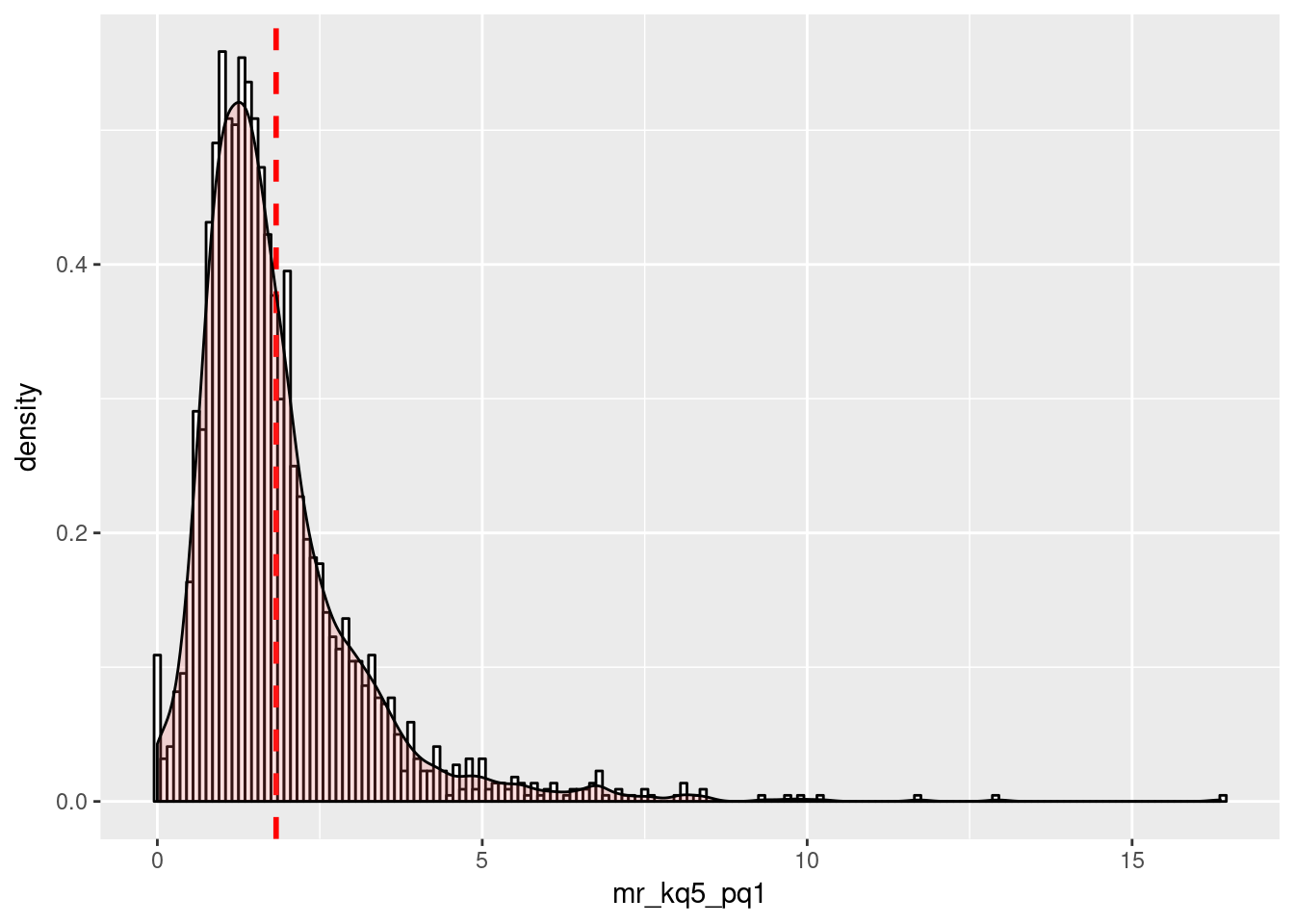

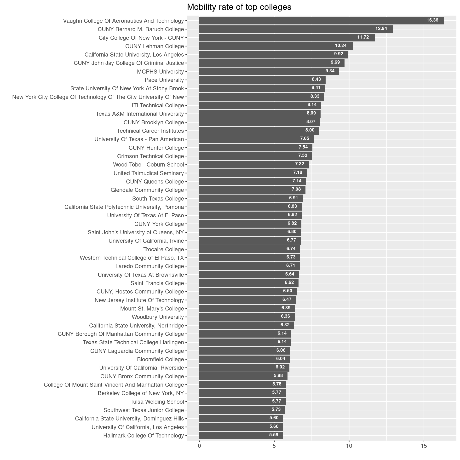
So what were the schools that were in the top 50 of ratings?

library(forcats)
ratings %>% 
  arrange(-mr_kq5_pq1) %>%
  select(name, mr_kq5_pq1) %>%
  head(50) %>%
  ggplot(aes(fct_reorder(as.factor(name), mr_kq5_pq1), mr_kq5_pq1)) + 
    geom_bar(stat='identity') + 
    labs(title="Mobility rate of top colleges") +
    xlab('') +
    ylab('') +
    geom_text(aes(label=sprintf('%0.2f', mr_kq5_pq1)), 
              hjust=1.5,
              vjust=0.25,
              size=2.5,
              position = position_dodge(width = 1), 
              colour="white",
              fontface = "bold",
              inherit.aes = TRUE) +
    coord_flip()